Page 69 - 2021-bfw-SPA-4e-TE-sample.indd

150 CHAPTER 2 • M o deling One - V ariable Quan tita tiv e Da ta
150

CHAPTER 2 • Modeling One-Variable Quantitative Data
TEACHING TIP Chapter 2 Review Exercises
Remind your students to watch the

Review Exercise videos, indicated by 1. Your Iowa home (2.1) The following dotplot gives the points that are 1, 2, and 3 standard deviations from

sale prices for 40 houses in Ames, Iowa, sold during a
the mean.
the play button icon . Students can recent month. The mean sale price was $203,388 with (b) Use the empirical rule to estimate the percentage of

find these videos in the resources on the a standard deviation of $87,609. horse pregnancies that are longer than 342 days.

digital platform or on the Student site at d d d d dd d d d dd d dd d d d d d d dd dd d dd 5. Density of the earth (2.4) In 1798, the English scientist
ddd
d dd d
d dd
ddd
bfwpub.com/spa4e. 50 100 150 200 250 300 350 400 450 Henry Cavendish measured the density of the earth
several times by careful work with a torsion balance.
Price ($1000s) The variable recorded was the density of the earth as a
multiple of the density of water. Here are Cavendish’s

(a) Find the percentile of the house represented by the 29 measurements, along with a dotplot and numeri-
FULL SOLUTIONS TO CHAPTER 2 red dot. cal summaries of the data.
29
(b) Calculate and interpret the standardized score ( z -score)

REVIEW EXERCISES for the house represented by the red dot, which sold 5.50 5.61 4.88 5.07 5.26 5.55 5.36 5.29 5.58 5.65
for $234,000. 5.57 5.53 5.62 5.29 5.44 5.34 5.79 5.10 5.27 5.39

You can nd the full solutions to the (c) The same house sold 5 years earlier for $212,500.

Chapter 2 Review Exercises by clicking During the month when this occurred, the mean sales 5.42 5.47 5.63 5.34 5.46 5.30 5.75 5.68 5.85
on the link in the TE-book or by logging price of homes in Ames, Iowa, was $191,223 with a d d d d d d d d d d d d d d d d d d d d d d d d d d d d d
standard deviation of $76,081. In which of the two
into the teachers’ resources on our digital years did the house sell for more money, relatively 4.9 5.0 5.1 5.2 5.3 5.4 5.5 5.6 5.7 5.8
platform. speaking? Explain your answer. Density of earth
2. Transforming data (2.2) The distribution of employee n Mean SD Min Q 1 Med Q 3 Max

salary at a large company is skewed to the right, 29 5.448 0.221 4.88 5.295 5.46 5.615 5.85
Answers to Chapter 2 Review with mean $75,100 and standard deviation $36,554.
Because the company had a productive year, the CEO
Exercises will give every employee 2% of their annual salary as a Is this distribution approximately normal? Justify your

answer based on the graph and the empirical rule.
year-end reward, along with a $500 Christmas bonus.

1. (a) There are 26 homes that sold for So an employee with a $60,000 salary would receive 6. Acing the GRE (2.5, 2.6) The Graduate Record Exam-
an adjusted salary of (60,000)(1.02) 500+
=

.
$61,700

inations (GREs) are widely used to help predict the
less than $234,000. This home’s selling (a) What shape would the distribution of adjusted salary performance of applicants to graduate schools. The

price is at the 65th percentile. have? Explain your answer. scores on the GRE Chemistry test are approximately
normal with mean 694 and standard deviation 112.

234,000 −203,388 (b) Find the mean of the distribution of adjusted salary. (a) About what percent of test takers earn a score less

(b) z = = 0.35 (c) Find the standard deviation of the distribution of than 500 on the GRE Chemistry test?
87,609 adjusted salary. (b) What proportion of test takers earn a score greater

This home has a sale price that is 0.35 3. Fetch, Bucket! (2.3) Kristen likes to throw tennis balls than or equal to 900 on this test?
standard deviations above the mean sale for her dog, Bucket. The time it takes Bucket to chase (c) Estimate the score at the 99th percentile on the GRE

down a ball, return to Kristen, and drop the ball at her
price. feet is equally likely to take any value in the interval Chemistry test.
from 8 seconds to 15 seconds.

(c) 5 years earlier: (a) Draw a density curve to model this distribution. Be 7. Ketchup (2.5, 2.6) A fast-food restaurant has just
installed a new automatic ketchup dispenser for use

212,500 −191,223 sure to include scales on both axes. in preparing its burgers. The amount of ketchup dis-
z = (C) 2021 BFW Publishers -- for review purposes only.
= 0.28
pensed by the machine follows an approximately

76,081 (b) About what proportion of the time will Bucket return normal distribution with mean 1.05 fluid ounces and
the ball within 13 seconds?

The house sold for more money recently (c) What is the mean of the density curve in part (a)? standard deviation 0.08 fluid ounce.

because the z-score for the recent selling Explain your reasoning. (a) If the restaurant’s goal is to put between 1 and 1.2
ounces of ketchup on each burger, about what percent
price z =( 0.35) is greater than the z-score 4. Horse pregnancies (2.3, 2.4) Bigger animals tend to of the time will this happen?

for the selling price 5 years earlier z =( 0.28). carry their young longer before birth. The length of (b) Suppose that the manager adjusts the machine’s set-
horse pregnancies from conception to birth varies
tings so that the mean amount of ketchup dispensed
2. (a) Skewed to the right, just according to a roughly normal distribution with mean is 1.1 ounces. How much does the machine’s standard
336 days and standard deviation 6 days.
like the original distribution (a) Sketch the normal curve that models the distribution deviation have to be reduced to ensure that at least
99% of the restaurant’s burgers have between 1 and

(b) Mean (75,100)(1.02) 500= + = $77,102 of horse pregnancy length. Label the mean and the 1.2 ounces of ketchup on them?
=
(c) SD (36,554)(1.02) $37,285.08
=
3. (a)
Height = 1
7
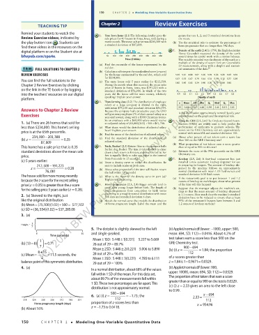
5. The dotplot is slightly skewed to the left (ii) Applet/normalcdf(lower:–1000,upper: 500, 07/09/20 1:59 PM
03_StarnesSPA4e_24432_ch02_088_153.indd 150
=
8 15 and single-peaked. mean: 694,SD: 112)0.0416. About 4.2% of
Time (seconds) Mean 1SD: 5.448 1(0.221)5.227 to 5.669 test takers earn a score less than 500 on the
±
±
−
(b) (138)   1 = 0.71 26 outof29 89.7%= GRE Chemistry test.
 
  7
−694
900
±
±
+
815 Mean 2SD: 5.448 2(0.221)5.006 to 5.890 (b) (i) z = 112 =1.84; the proportion
=
(c) Mean = =11.5 seconds, the 28 outof29 96.6%
2 Mean 3SD: 5.448 3(0.221)4.785 to 6.111 of z-scores greater than
±
±
=
balance point of this symmetric distribution. 29 outof29 100% z =1.84 is1–0.9671 0.0329.
=
4. (a) In a normal distribution, about 68% of the values (ii) Applet/normalcdf(lower: 900,
=
fall within 1 SD of the mean. For this data set, upper:10000,mean: 694,SD:112)0.0329.
about 89.7% of the measurements fall within The proportion of test takers that earn a score
1 SD. These two percentages are far apart. This greater than or equal to 900 on the test is 0.0329.
distribution is not approximately normal. (c) (i) z = 2.33 gives an area to the left close
to 0.99.
500 −694
6. (a) (i) z = =−1.73; the 2.33 = x − 694
318 324 330 336 342 348 354 112 112
Horse pregnancy length (days) proportion of z-scores less than x = 954.96
(b) About 16% z = –1.73 is 0.0418.
150 CHAPTER 2 • Modeling One-Variable Quantitative Data
03_TysonTEspa4e_25177_ch02_088_153_4pp.indd 150 10/11/20 7:49 PM