Page 65 - 2021-bfw-SPA-4e-TE-sample.indd

146 CHAPTER 2 • Modeling One-Variable Quantitative Data

21. The normal probability plot is fairly 23. Normal outliers In Chapter 1, you learned the
linear, indicating that the distribution Extending the Concepts 1.5× IQR rule to identify outliers. We call a data
of heart rate for the 200 male runners is Exercises 21 and 22 refer to the following. A type of value an outlier if it is less than Q 1 − 1.5× IQR
graph called a normal probability plot (or a normal
1.5× IQR. In the final match
3 +
or greater than Q
approximately normal. quantile plot) can be used to assess whether or not a of the 2018 Australian Open tennis tournament,
distribution of quantitative data is approximately nor- champion Roger Federer had a mean speed of
22. The normal probability plot is clearly mal. This graph consists of a point for each individual in 188 kilometers per hour (kph) on his first serves.
curved, indicating that the distribution of the data set. The x-coordinate of each point is the actual Assuming that the distribution of his first-serve
CO 2 emissions for the 48 countries is not data value, and the y-coordinate is the expected z-score speeds is roughly normal with a standard devi-
ation of 7 kph, what speeds qualify as high
in a standard normal distribution corresponding to the
approximately normal. percentile of that data value. If the points on a normal outliers?
probability plot lie close to a straight line, the data are
23. Qz = –0.67 gives an area to the approximately normally distributed. A clear nonlin- Recycle and Review
: 1
left of about 0.25: −0.67 =− ear form in a normal probability plot indicates a non- 24. Chamois clean? (1.8) Chamois leather is smooth
x 188/7;
x =183.31 normal distribution. You can use the TI-83/84 to make and absorbent, making it a popular choice for use
a normal probability plot for a quantitative data set. in cleaning. Does the temperature of the water
(ii) invNorm(area: 0.25,mean:188, 21. Runners’ heart rates The figure shows a normal affect how much it can absorb? An inquisitive stu-
=
SD:7) 183.28 kph. probability plot of the heart rates of 200 male run- dent cut out 90 3-inch-by-3-inch squares of cham-
ois leather and randomly assigned 30 to be used
26
ners after 6 minutes of exercise on a treadmill. with hot water, 30 with room temperature water,
Q 3 : (i) z = 0.67 gives an area to the left of Use the graph to determine if this distribution of and 30 with cold water. After soaking each piece
28
x 188/7;
about 0.75: 0.67 =− x =192.69 heart rates is approximately normal. with the appropriate temperature water, the stu-
dent carefully measured how much water was
(ii) invNorm(area: 0.75,mean:188, 3 d absorbed (in milliliters) by wringing out each
SD:7) 192.72 kph. 2 d d d d piece of leather over a graduated cylinder. The
=
d d d d d boxplots display the distribution of amount of
d d d d
Q =183.3 and Q =192.7. 1 d d d d d d d d d d d d d d water absorbed for each of these types. Compare
1
3
these distributions.
IQR =192.7–183.3 9.4kph d d d d d d d d d d d d d d d d d d d d d 27review purposes only.
=
Highoutlier >192.71.5(9.4) 206.8kph Expected z-score 0 d d d d d d d d d d d d d d d d d d d d d d Hot
+
=
First-serve speeds that exceed 206.8 kph –1 d d d d d d d d d d d d d d d d d d d Temperature Room
qualify as high outliers. –2 d d d d d d d d d d d d d d Cold
d d
24. The shape is slightly skewed to the –3 d 1 2 3 4 5 6 7 8
right for all three temperatures. The cold 70 80 90 100110 120130 140150 Amount of water absorbed (ml)
temperature distribution contains a high Heart rate (beats per minute) 25. Is North Carolina normal? (2.3, 2.4) We collected
(C) 2021 BFW Publishers -- for
outlier. The other distributions do not 22. Carbon dioxide emissions The figure shows a nor- data on the tuition charged by colleges and univer-
sities in North Carolina. Here are some numerical
mal probability plot of the emissions of carbon
contain any outliers. The median amount dioxide per person in 48 countries. Use the graph summaries for the data:
of water absorbed is greatest for the to determine if this distribution of carbon dioxide Mean SD Min Max
emissions is approximately normal.
hot temperature (about 4.9 mL), is less 3 14,281.86 11,212.71 4216 54,430
for the room temperature distribution d (a) Sketch a normal distribution with mean 14,281.86
(about 3.2 mL), and is even less for the 2 d d d d and standard deviation 11,212.71. Label the mean
cold temperature distribution (about 1 d d d d d d d d d d d d d and the points that are 1, 2, and 3 standard devia-
tions from the mean.
1.2 mL). The variability in amount of Expected z-score 0 d d d d d d d d d d d d d d d d d d (b) Based on your graph in part (a) and the summary
water absorbed is greatest for the room –1 d d d d d d d d d d d d statistics, is it reasonable to believe that the distri-
temperature distribution IQR ≈( 1.6mL), –2 d d d bution of North Carolina tuitions is approximately
normal? Explain your reasoning.
is slightly less for the hot temperature –3
distribution IQR ≈( 1.3mL), and is slightly 0 2 4 6 8 10 12 14 16 18 20
CO 2 emissions
less for the cold temperature distribution (metric tons per person)
( IQR ≈1.2mL).
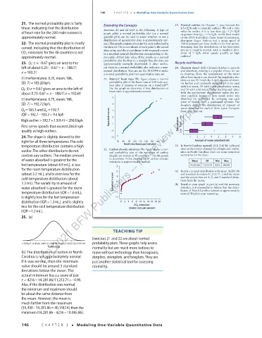
25. (a)
TEACHING TIP
03_StarnesSPA4e_24432_ch02_088_153.indd 146 07/09/20 1:58 PM
Exercises 21 and 22 are about normal
–19356.27–8143.56 3069.1514281.86 25494.5736707.28 47919.99 probability plots. These graphs help assess
Tuition ($) normality but are much more tedious to
(b) The distribution of tuition in North make without technology than histograms,
Carolina is not approximately normal. dotplots, stemplots, and boxplots. They are
If it was normal, then the minimum just another statistical tool for assessing
value should be around 3 standard normality.
deviations below the mean. The
actual minimum has a z-score of just
−
z = 4216 14,281.86/11,212.71 –0.90.
=
Also, if the distribution was normal,
the minimum and maximum should
be about the same distance from
the mean. However, the mean is
much farther from the maximum
(54,430–14,281.86 40,148.14) than the
=
minimum (14,281.86– 4216 10,065.86)= .
146 CHAPTER 2 • Modeling One-Variable Quantitative Data
03_TysonTEspa4e_25177_ch02_088_153_4pp.indd 146 10/11/20 7:49 PM