Page 18 - 2021-bfw-SPA-4e-TE-sample.indd

LESSON 2.2 • Transforming Data 99

EXAMPLE

How wide is this room?
Effect of adding/subtracting a constant

PROBLEM: Soon after the metric system was introduced in NoSystem images/E+/Getty Images Lesson 2.2
Australia, a group of students was asked to guess the width
of their classroom to the nearest meter. Here is a dotplot of
the data along with some numerical summaries.
The actual width of the room was 13 meters. We can
examine the distribution of students’ errors by defining

a new variable as follows: errorguess 13= − . Note
that a negative value for error indicates that a
student’s guess for the width of the room was
too small.
(C) 2021 BFW Publishers -- for review purposes only.

(a) What shape would the distribution of error have?
0 10 20 30 40
(b) Find the mean and median of the distribution
of error. − Guess (m)
(c) Find the standard deviation and interquartile n x s x Min Q 1 Med Q 3 Max IQR Range

range of the distribution of error. Guess 44 16.02 7.14 8 11 15 17 40 6 32
SOLUTION:

(a) The same shape as the original distribution of guesses: skewed Subtracting 13 from each data value doesn’t
to the right with two distinct peaks. change the shape of the distribution.
(b) Mean:16.02 −13 =3.02meters; It is not a surprise that the mean is greater than
the median in this right-skewed distribution.
−
=
M edian:15 13 2meters.

(c) Standard deviation: 7.14 meters; IQR : 6 meters. Subtracting a constant doesn’t affect measures
of variability.
FOR PRACTICE TRY EXERCISE 5.

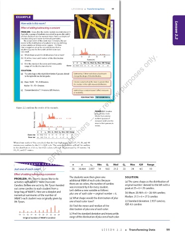
Figure 2.2 confirms the results of the example.
FIGURE 2.2 Dotplots
Guess (m) d d d d d d d d d d d d d d d d d d d d d d d d d d and summary statis-
tics for the Australian
students’ guesses of
d
d
d
d
d
d
d
d
d
d
d
d
d
d
d
d
d
d
classroom width and the
d
Error (m) ddddddddddd dd dd d d d errors in their guesses, in
d
d
d
d
d
dd
dd
meters.
dd ddddd
ddddddddd
0 10 20 30 40
n − x s x Min Q 1 Med Q 3 Max IQR Range
Guess (m) 44 16.02 7.14 8 11 15 17 40 6 32
Error (m) 44 3.02 7.14 –5 –2 2 4 27 6 32
What about outliers? You can check that the four highest guesses—27, 35, 38, and 40
meters—are outliers by the 1.5 × IQR rule. The same individuals will still be outliers

in the distribution of error, but their values will each be decreased by 13 meters: 14,
22, 25, and 27 meters.
03_StarnesSPA4e_24432_ch02_088_153.indd 99 07/09/20 1:54 PM
AL TERNA TE EX AMPLE n x s x Min Q 1 Med Q 3 Max IQR Range
Just one of each color? 28 20.464 2.937 14 18.5 21.5 23 24 4.5 10
Effect of adding/subtracting a constant
The students were then given one SOLUTION:
PROBLEM: Mr. Tyson’s classes like to do
activities with M&M’S® Milk Chocolate additional M&M of each color. Because (a) The same shape as the distribution of
Candies. Before one activity, Mr. Tyson handed there are six colors, the number of candies original number: skewed to the left with a
+=
out some candies to each student from a was increased by 6 for every student. peak at 236 29 candies.
large bag of M&M’S. Here are a dotplot and Let’s define a new variable as follows: (b) Mean: 20.464 6 26.464 candies;+=
+
numerical summaries of the number of plusone of each color = originalnumber 6. Median: 21.56 27.5candies
+=
M&M’S each student was originally given by (a) What shape would the distribution of plus
Mr. Tyson. one of each color have? (c) Standard deviation: 2.937 candies;
(b) Find the mean and median of the IQR: 4.5 candies
distribution of plus one of each color.
(c) Find the standard deviation and interquartile
14 15 16 17 18 19 20 21 22 23 24
Original number of M&M’S (candies) range of the distribution of plus one of each color.
LESSON 2.2 • Transforming Data 99
03_TysonTEspa4e_25177_ch02_088_153_4pp.indd 99 10/11/20 7:43 PM