Page 15 - 2021-bfw-SPA-4e-TE-sample.indd

96 CHAPTER 2 • Modeling One-Variable Quantitative Data

19. The speed limit is set at the value of major league batting averages has changed over
that will have 85% of the vehicles on that the years. The distributions are quite symmetric,
road traveling at a speed less than the except for outliers such as Cobb, Williams, and
Brett. While the mean batting average has been held
580
575
570
speed limit. roughly constant by rule changes and the balance 565 Long-jump distance (cm) 585
between hitting and pitching, the standard deviation
20. The 90th percentile means that 90% has dropped over time. Here are the facts: 6 n Mean SD Min Q 1 Med Q 3 Max
of men like Larry have cholesterol levels 40 577.3 4.713 564 574.5 577 581.5 586
that are lower than his. When it comes to Decade Mean Standard deviation (a) Sedona was one of the athletes at this meet. Her
0.0371
1910s
0.266
cholesterol, a high number is not desirable. 1940s 0.267 0.0326 best long jump measured 571 centimeters. Find
Sedona’s percentile. Interpret this value.
21. (a) 27/300.9. Connor’s head 1980s 0.261 0.0317 (b) Find and interpret the standardized score (z-score)
=
circumference is at the 90th percentile. Who had the best performance for the decade he for Sedona’s best long jump.
90% of players on the team have a played? Explain your reasoning. (c) In the distribution of high jump performances at
the meet, Sedona’s z-score was −1.03. Which of her
(C) 2021 BFW Publishers -- for review purposes only.
smaller head circumference than Connor. Applying the Concepts jumps was better? Explain your reasoning.
24 −22.697 23. Big or little? Mrs. Munson wants to know how
(b) z = =1.22. Connor’s head 19. Setting speed limits According to the Los Angeles her son’s height and weight compare with those of
1.07 Times, speed limits on California highways are set other boys his age. She uses an online calculator to
circumference is 1.22 standard deviations at the 85th percentile of vehicle speeds on those determine that her son is at the 48th percentile for
stretches of road. Explain to someone who knows
above the mean head circumference. little statistics what that means. weight and the 76th percentile for height. Explain
to Mrs. Munson what these values mean.
(c) Yes, because Connor’s z-score for head 20. Percentile pressure Larry came home very excited after 24. Run faster Peter is a star runner on the track team. In
circumference z =( 1.22) is greater than a visit to his doctor. He announced proudly to his wife, the league championship meet, Peter records a time
“My doctor says my cholesterol level is at the 90th
his z-score for height z =( 0.87). percentile among men like me. That means I’m bet- that would fall at the 80th percentile of all of his
race times that season. But his performance places
ter off than about 90% of similar men.” How should him at the 50th percentile in the league champion-
22. (a) 3/400.075. Sedona’s best his wife, who has taken statistics, respond to Larry’s ship meet. Explain how Peter’s performances com-
=
long jump is at the 7th percentile. statement? pare. (Remember that shorter times are better in this
7% of the athletes at the meet had a 21. Wear your helmet! Many athletes (and their parents) scenario!)
best long jump that is less than Sedona’s. worry about the risk of concussions when playing Extending the Concepts
sports. A football coach plans to obtain specially
571 −577.3 made helmets for his players that are designed to A cumulative relative frequency graph plots a point corre-
(b) z = =−1.34. Sedona’s best reduce the chance of getting a concussion. Here are sponding to the percentile of a given value in a distribution
4.713 a dotplot and numerical summaries of the head cir- of quantitative data. Consecutive points are then con-
long jump is 1.34 standard deviations below cumference (in inches) of each player on the team. nected with a line segment to form the graph. This graph
can be used to describe the location of an individual value
the mean of the athlete’s best long jumps. d d d dd ddd d ddd dddddd d dd d d d d d dd d d in a distribution or to find a specific percentile of the dis-
(c) High jump, because her z-score for the 21 21.5 22 22.5 23 23.5 24 24.5 25 25.5 tribution. Exercises 25 and 26 involve cumulative relative
frequency graphs.
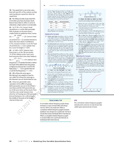
high jump =z( –1.03) is greater than her Head circumference (in.) 25. Household income The cumulative relative fre-
z-score for the long jump =z( –1.34). n Mean SD Min Q 1 Med Q 3 Max quency graph describes the distribution of median
30 22.697 1.07 20.8 22 22.65 23.4 25.6 household incomes in the 50 states in 2018. 7
23. 48% of boys the same age as
Mrs. Munson’s son weigh less than her (a) Connor, the team’s starting quarterback, has a 100
head circumference of 24.0 inches. Find Connor’s
son, while 76% of boys the same age as percentile. Interpret this value. 80
Mrs. Munson’s son are shorter than her son. (b) Find and interpret the standardized score (z-score) 60
for Connor’s head circumference.
24. These two percentiles were (c) In the distribution of players’ heights, Connor’s Percentile
calculated within different groups z-score is 0.87. Is Connor’s head circumference rel- 40
atively large for his height? Explain your reasoning.
(80th percentile was out of all of Peter’s 22. Long jump There were 40 athletes competing in the 20
race times and the 50th percentile was long jump at a major track meet. The meet official 0
out of all racers’ times at this meet). Peter recorded the distance, to the nearest centimeter, of 40 50 60 70 80 90
each athlete’s best jump. Here are a dotplot and some
must be a star runner because even numerical summaries of the data. Median household income ($1000s)
when he isn’t having one of his personal
best performances, he is still racing in
the middle of the pack at the league
championship meet. 03_StarnesSPA4e_24432_ch02_088_153.indd 96 FYI 07/09/20 1:54 PM
TEACHING TIP
The cumulative relative frequency graphs
A cumulative relative frequency graph always
increases or stays constant (flat) and always introduced in exercises 25 and 26 are also
reaches 100% as its maximum. When a called ogives (pronounced oh-jive).
cumulative relative frequency graph increases
quickly (is very steep) over a particular interval, it
reveals that many individuals fall in that interval.
When a cumulative relative frequency graph
is constant (flat) over a particular interval, no
individuals fall in that interval.

96 CHAPTER 2 • Modeling One-Variable Quantitative Data

03_TysonTEspa4e_25177_ch02_088_153_4pp.indd 96 10/11/20 7:43 PM