Page 25 - 2021-bfw-SPA-4e-TE-sample.indd

106 CHAPTER 2 • Modeling One-Variable Quantitative Data

=
=
+
15. (a) Mean ($9)(0.15) $2 $2.35 15. Big tipper? When Sam goes to a restaurant, he 18. Large fries Ryan and Brent were curious about the
(b) SD ($3)(0.15) $0.45 always tips the server $2 plus 15% of the cost of the amount of french fries they would get in a large
=
=
meal. Suppose that Sam’s distribution of meal costs order from their favorite fast-food restaurant,
+
=
16. (a) Median (4.600.1)1.2 5.64 has a mean of $9 and standard deviation of $3. Burger King. They went to several different Burger
=
×
=
(b) IQR = 2.10 ×1.22.52 (a) Find the mean of his distribution of tip amount. King restaurants over a series of days and ordered
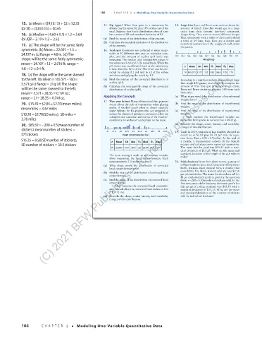
(b) Calculate the standard deviation of his distribution a total of 14 large fries. Here are a doplot and
17. (a) The shape will be the same: fairly of tip amount. numerical summaries of the weight of each order
+
=
symmetric. (b) Mean22.6971.5 = 16. Acid rain? Rainwater was collected in water recep- (in grams). d d d
d
d
d
d
d
=
24.197in. (c) Range4.8in. (d) The tacles at 30 different sites near an industrial com- 152 154 156 158 d 160 162 d 164 d 166 d 168 170 d 172 d
shape will be the same: fairly symmetric; plex, and the amount of acidity (pH level) was Weight (g)
measured. The median and interquartile range of
mean = 24.197 ÷12 2.016 ft;range = the values are 4.60 and 2.10, respectively. When the
=
=
4.8 ÷12 0.4ft. pH meter was recalibrated back at the laboratory, n Mean SD Min Q 1 Med Q 3 Max
it was found to be in error. The error can be cor-
rected by adding 0.1 pH unit to all of the values 14 165.571 5.571 152 163 166.5 170 173
18. (a) The shape will be the same: skewed and then multiplying the result by 1.2.
(C) 2021 BFW Publishers -- for review purposes only.
=
to the left. (b) Mean165.571–160 = (a) Find the median of the corrected distribution of According to a nutrition website, Burger King’s large
5.571g (c) Range21g (d) The shape acidity (pH). fries weigh 160 grams, on average. To compare the
=
will be the same: skewed to the left; (b) Calculate the interquartile range of the corrected amount of fries they got to Burger King’s claim,
distribution of acidity (pH).
Ryan and Brent decide to subtract 160 from each
=
÷
mean = 5.571 28.35 0.197 oz; data value.
range21 ÷28.35 0.741oz. Applying the Concepts (a) What shape would the distribution of transformed
=
=
17. Wear your helmet! Many athletes (and their parents) weights have?
19. $15.45 $2.85 $2.70(meanmiles); worry about the risk of concussions when playing (b) Find the mean of the distribution of transformed
+
=
meanmiles4.67miles sports. A football coach plans to obtain specially weights.
=
made helmets for his players that are designed to (c) Find the range of the distribution of transformed
$10.20 = $2.70(SDmiles); SDmiles = reduce the chance of getting a concussion. Here are weights.
Now suppose the transformed weights are
3.78miles a dotplot and numerical summaries of the head cir- converted from grams to ounces (1 oz = 28.35 g).
cumference (in inches) of each player on the team.
+
=
20. $85.50 –200 0.5(meannumber of d d ddd d d d (d) Describe the shape, center (mean), and variability
stickers); meannumber of stickers = 21 d d 21.5 22 dd ddd 22.5 dddddd 23 dd d 23.5 d 24 dd d 24.5 25 25.5 d (range) of this distribution.
d
571stickers Head circumference (in.) 19. Taxi! In 2019, taxicabs in Los Angeles charged an
initial fee of $2.85 plus $2.70 per mile. In equa-
+
$15.25 = 0.50(SDnumberofstickers); n Mean SD Min Med Max tion form, Fare = 2.85 2.7(miles). At the end of
a month, a businessman collects all his taxicab
SDnumber of stickers = 30.5stickers Q 1 Q 3 receipts and calculates some numerical summaries.
30 22.697 1.07 20.8 22 22.65 23.4 25.6 The mean fare he paid was $15.45 with a stan-
dard deviation of $10.20. What are the mean and
standard deviation of the length of his cab rides in
The team manager made an unfortunate mistake miles?
when measuring the head circumferences: Each
measurement is 1.5 inches too small. 20. Sticky business From their dorm rooms, a group of
(a) What shape would the distribution of corrected college students runs a small company selling water
head circumference have? bottle stickers. Each student buys a printer that
(b) Find the mean of the distribution of corrected head costs $200. The blank stickers and ink cost $0.50
per printed sticker. The water bottle stickers sell for
circumference. $1, so each student’s profit is given by the equation
(c) Find the range of the distribution of corrected head Profit =−200 0.50(numberofstickerssold). In the
+
circumference. first two years of the business, the mean profit for
Now suppose the corrected head circumfer- this group of college students was $85.50 with a
ence of each player is converted from inches to feet standard deviation of $15.25. What are the mean
(1 ft = 12 in.). and standard deviation of the number of stickers
(d) Describe the shape, center (mean), and variability sold by individual students?
(range) of this distribution.
03_StarnesSPA4e_24432_ch02_088_153.indd 106 07/09/20 1:55 PM
106 CHAPTER 2 • Modeling One-Variable Quantitative Data

03_TysonTEspa4e_25177_ch02_088_153_4pp.indd 106 10/11/20 7:44 PM