Page 28 - 2021-bfw-SPA-4e-TE-sample.indd

LESSON 2.3 • Density Curves and the Normal Distribution 109

the bookstore took less than 4 minutes. That’s 669/1000 = 0.669 = 66.9% —very close

to the estimate we got using the density curve. AL TERNA TE EX AMPLE
Recall from Chapter 1 that we can describe the distribution of journey times in

Figure 2.5(a) as approximately uniform. The density curve in Figure 2.5(b) is called a When will an enemy appear?
uniform density curve because it has constant height.
Modeling with density curves
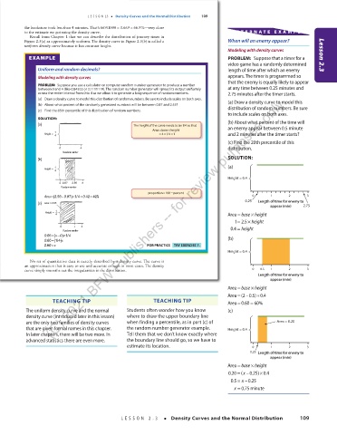
EXAMPLE PROBLEM: Suppose that a timer for a Lesson 2.3
video game has a randomly determined
Uniform and random decimals? length of time after which an enemy
Modeling with density curves appears. The timer is programmed so
that the enemy is equally likely to appear
PROBLEM: Suppose you use a calculator or computer random number generator to produce a number

between 0 and 4 (like 0.84522 or 3.1111119). The random number generator will spread its output uniformly at any time between 0.25 minutes and
across the entire interval from 0 to 4 as we allow it to generate a long sequence of random numbers. 2.75 minutes after the timer starts.
(C) 2021 BFW Publishers -- for review purposes only.
(a) Draw a density curve to model this distribution of random numbers. Be sure to include scales on both axes. (a) Draw a density curve to model this

(b) About what percent of the randomly generated numbers will be between 0.87 and 2.55? distribution of random numbers. Be sure

(c) Find the 65th percentile of this distribution of random numbers.

to include scales on both axes.
SOLUTION:
(a) The height of the curve needs to be 1/4 so that (b) About what percent of the time will

×
Area = base height an enemy appear between 0.5 minute
Height = 1 =× =1 and 2 minutes after the timer starts?
41/4
4
(c) Find the 20th percentile of this
0 4 distribution.
Random number
SOLUTION:
(b)
Height = 1 (a)
4
Height = 0.4
0 0.87 2.55 4
Random number
=
proportion ×100 percent

−
=
=
Area =(2.550.87) ×1/40.42 42% 0 1 2 3
0.25 Length of time for enemy to
(c) Area = 0.65
appear (min) 2.75
1
×
Height =
4 Area = base height
1 = 2.5 × height
0 x 4 0.4 = height
Random number
=− ×
0.65 (x 0)1/4 (b)
0.65 =(1/4)x
2.60 =x FOR PRACTICE TRY EXERCISE 7.
Height = 0.4
No set of quantitative data is exactly described by a density curve. The curve is
an approximation that is easy to use and accurate enough in most cases. The density
curve simply smooths out the irregularities in the distribution. 0 0.5 1 2 3
Length of time for enemy to
appear (min)
×
Area = base height
×
Area = (2–0.5)0.4
03_StarnesSPA4e_24432_ch02_088_153.indd 109 07/09/20 1:55 PM
TEACHING TIP TEACHING TIP Area = 0.60 60%
=
The uniform density curve and the normal Students often wonder how you know (c)
density curve (introduced later in this lesson) where to draw the upper boundary line
are the only two families of density curves when finding a percentile, as in part (c) of Area = 0.20
that are given formal names in this chapter. the random number generator example. Height = 0.4
In later chapters, there will be two more. In Tell them that we don’t know exactly where
advanced statistics there are even more. the boundary line should go, so we have to
estimate its location. 0 1 2 3
0.25 Length of time for enemy to
appear (min)
×
Area = base height
=
×
0.20( x –0.25) 0.4
0.5 = x –0.25
x = 0.75 minute
LESSON 2.3 • Density Curves and the Normal Distribution 109
03_TysonTEspa4e_25177_ch02_088_153_4pp.indd 109 10/11/20 7:44 PM