Page 31 - 2021-bfw-SPA-4e-TE-sample.indd

112 CHAPTER 2 • Modeling One-Variable Quantitative Data

that the student’s performance is typical for a student in the third month of grade 6.
The histogram is roughly symmetric, and both tails fall off smoothly from a single
center peak. There are no large gaps or obvious outliers.
The density curve drawn through the tops of the histogram bars in Figure 2.9(b) is a
FYI good description of the overall pattern of the ITBS score distribution. We call it a normal
Normal distributions are also called curve. The distributions described by normal curves are called normal distributions. In
this case, the ITBS vocabulary scores of Gary, Indiana, seventh- graders are approxi-
Gaussian distributions in honor of Karl mately normally distributed.
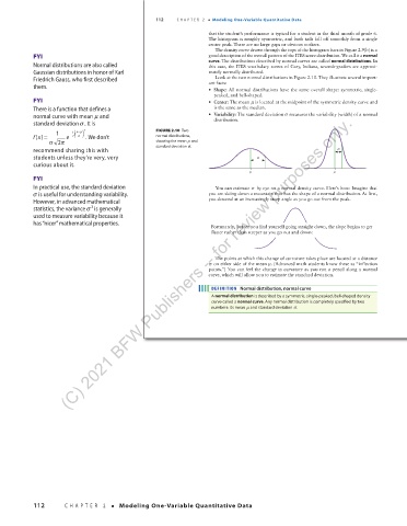
Friedrich Gauss, who first described Look at the two normal distributions in Figure 2.10. They illustrate several import-
them. ant facts:
• Shape: All normal distributions have the same overall shape: symmetric, single-
peaked, and bell-shaped.
FYI • Center: The mean µ is located at the midpoint of the symmetric density curve and
There is a function that defines a is the same as the median.
(C) 2021 BFW Publishers -- for review purposes only.
normal curve with mean µ and • Variability: The standard deviation σ measures the variability (width) of a normal
standard deviation σ . It is distribution.
x µ
1 − 1 ( ) 2 FIGURE 2.10 Two
−
fx = e 2 σ . We don’t normal distributions,
()
σ 2 π showing the mean µ and
recommend sharing this with standard deviation σ.
students unless they’re very, very
curious about it.
FYI
In practical use, the standard deviation You can estimate σ by eye on a normal density curve. Here’s how: Imagine that
σ is useful for understanding variability. you are skiing down a mountain that has the shape of a normal distribution. At first,
However, in advanced mathematical you descend at an increasingly steep angle as you go out from the peak.
2
statistics, the variance σ is generally
used to measure variability because it
has “nicer” mathematical properties.
Fortunately, before you find yourself going straight down, the slope begins to get
flatter rather than steeper as you go out and down:

The points at which this change of curvature takes place are located at a distance
σ on either side of the mean µ. (Advanced math students know these as “inflection
points.”) You can feel the change in curvature as you run a pencil along a normal
curve, which will allow you to estimate the standard deviation.
DEFINITION Normal distribution, normal curve
A normal distribution is described by a symmetric, single-peaked, bell-shaped density
curve called a normal curve. Any normal distribution is completely specified by two
numbers: its mean µ and standard deviation σ .

03_StarnesSPA4e_24432_ch02_088_153.indd 112 07/09/20 1:55 PM

112 CHAPTER 2 • Modeling One-Variable Quantitative Data

03_TysonTEspa4e_25177_ch02_088_153_4pp.indd 112 10/11/20 7:44 PM