Page 35 - 2021-bfw-SPA-4e-TE-sample.indd

116 CHAPTER 2 • Modeling One-Variable Quantitative Data

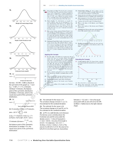
15. 15. Nine ounces of chips? The distribution of weight 20. Preheat before baking The time it takes a certain
pg 113 for 9-ounce bags of a particular brand of potato oven to preheat to 350 F° is equally likely to be any
chips can be modeled by a normal distribution value in the interval from 7 to 12 minutes.
with mean µ = 9.12 ounces and standard devia- (a) Draw a density curve that can be used to model this
tion σ = 0.05 ounce. Sketch the normal density distribution. Be sure to include scales on both axes.
curve. Label the mean and the points that are 1,
2, and 3 standard deviations from the mean. (b) What proportion of the time will the oven preheat
to 350º F in less than 8 minutes and 45 seconds?
8.97 9.02 9.07 9.12 9.17 9.22 9.27 16. Men’s heights The distribution of height for (c) Find the interquartile range of this distribution.
adult American men can be modeled by a nor -
Weight of 9-ounce bag of chips mal distribution with mean µ = 69 inches and (d) What is the mean of the density curve? Explain
your answer.
16. standard deviation σ = 2.5 inches. Sketch the (e) What is the median of the density curve? Explain
normal density curve. Label the mean and the
points that are 1, 2, and 3 standard deviations your answer.
from the mean. 21. A normal curve Estimate the mean and standard devi-
17. Rafa serves! Tennis superstar Rafael Nadal’s first ation of the normal density curve in the figure.
serve speeds (in miles per hour) in a recent season
can be modeled by a normal distribution with mean
115 mph and standard deviation 6 mph. Sketch
the normal density curve. Label the mean and the
points that are 1, 2, and 3 standard deviations from
61.5 64 66.5 69 71.5 74 76.5 the mean.
Height of adult American male
18. Cholesterol levels High levels of cholesterol in the 3 4 5 6 7 8 9 10 11 12 13 14 15 16 17
17. blood increase the risk of heart disease. Choles-
terol levels for 14-year-old boys can be modeled 22. Another normal curve Estimate the mean and stan-
by a normal distribution with mean 170 mg/dl dard deviation of the normal density curve in the
and standard deviation 30mg/dl. Sketch the nor- figure.
mal density curve. Label the mean and the points
that are 1, 2, and 3 standard deviations from the
mean.
97 103 109 115 121 127 133 Applying the Concepts
First serve speeds (mph)
19. Set the alarm Old-fashioned mechanical alarm 10 15 20 25 30 35 40 45 50
18. clocks were not very accurate about when the
alarm went off. Suppose that the alarm on one Extending the Concepts
such clock is equally likely to go off at any time 23. A weird density curve The figure shows a density
in the interval from 2 minutes before to 2 min-
utes after the time set for the alarm to go off. curve that models the distribution of a quantitative
Consider the distribution of the amount of time variable.
(in minutes) from when the alarm is set to go off 2
to when it actually goes off. Note that the value
of this variable will be negative if the alarm goes
80 110 140 170 200 230 260 off early.
Cholesterol levels (mg/dl)
(a) Draw a density curve that can be used to model 1
this distribution. Be sure to include scales on both
19. (a) 5 (C) 2021 BFW Publishers -- for review purposes only.
axes.
Height = 1 (b) What proportion of the time will the alarm go off
4
within 10 seconds of the time for which it is set?
–2 0 2 (c) Find the interquartile range of this distribution. 0 0.2 0.4 0.6 0.8 X
Amount of time (min) (d) What is the mean of the density curve? Explain Value
(b) Area 20/240 0.083 (c) Based on your answer. (a) Show that this is a valid density curve.
=
=
the symmetry in the graph, Q =1 and (e) What is the median of the density curve? Explain (b) About what proportion of the time would this
3
your answer.
Q = –1; IQR =1–(1)2minutes. variable take values between 0 and 0.2?
− =
1
=
(d) Mean 0minutes, the balance
point of this symmetric distribution.
=
(e) Median 0minutes, which is the
equal-areas point of this symmetric
distribution.
20. (a) 21. The estimate for the mean is 10. between =x 0.2 and = 0.4 is the equal- 07/09/20 1:55 PM
x
03_StarnesSPA4e_24432_ch02_088_153.indd 116
1 The curvature changes at 8 and 12, so 2 is areas point with an area of 0.50 to the left.
Height =
5 the estimate for the standard deviation. (d) Meanmedian due to the right-skewed
>
0 7 12 shape.
Time to preheat oven to 350°F 22. The estimate for the mean is 28.
=
(b) 45seconds 45/60 0.75minutes; The curvature changes at 23 and 33, so 5 is
=
 1 the estimate for the standard deviation.
area(8.75–7)   0.35 23. (a) This is a valid density curve because
=
=

=
(c) 1 =+Q 7(0.25)(5) 8.25; Q 3 = 7+ the density curve is entirely above the
(0.75)(5)10.75; IQR =10.75–8.25 = horizontal axis and the area under the
=
density curveis1. Area of trapezoid is
=
+
712
+
2.5minutes (d) mean = = 9.5, (1/2)(21)(0.4) = 0.6; area of rectangle is
2 (0.4)(1) = 0.4; totalarea 0.60.4 1.
+
=
=
the balance point of this symmetric (b) Area (1/2)(21.5)(0.2) 0.35 (c) The
=
=
+
distribution (e) median 9.5, the area to the left of 0.2 is 0.35. The area to the
=
equal-areas point of this symmetric left of 0.4 is 0.6 (from part (a)). Somewhere
distribution
116 CHAPTER 2 • Modeling One-Variable Quantitative Data
03_TysonTEspa4e_25177_ch02_088_153_4pp.indd 116 10/11/20 7:45 PM