Page 34 - 2021-bfw-SPA-4e-TE-sample.indd

LESSON 2.3 • Density Curves and the Normal Distribution 115

7. (a)
Mastering Concepts and Skills
Height = 1
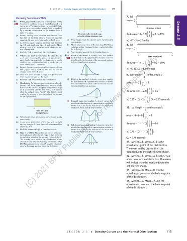
7. Biking accidents Researchers collected data on the 3
pg 109 location of accidents along a 3-mile bike path in a
tourist area. The distance from the start of the bike 0 3
path to where an accident occurred can be modeled Distance (miles)
by a uniform distribution on the interval from 0 –1 0 4 Lesson 2.3
miles to 3 miles. Time (min) after the bell rings (b) Area (1.1–0.8)   1 = 0.110%
=
=
  3
(a) Draw a density curve to model the distance from when Mr. Wilder dismisses class  
the start of the bike path to where an accident
=
occurred. Be sure to include scales on both axes. (a) What height must the density curve have? Justify (c) (0.7)(3) 2.1miles
(b) Aaliyah’s property adjoins the bike path between your answer.
the 0.8 mile mark and the 1.1 mile mark. About (b) About what proportion of the time does Mr. Wilder 8. (a)
what percent of accidents occurred along this sec- end class within 1 minute (before or after) of when 1
tion of the path? the bell rings? Height = 10
(C) 2021 BFW Publishers -- for review purposes only.
(c) Find the 70th percentile of this distribution. (c) Find the third quartile Q of this distribution.
3
8. Where’s the bus? Jayden takes the same bus to 11. Which is the mean? A density curve that models 0 Wait time (min) 10
work every morning. The amount of time (in min- pg 111 the distribution of a quantitative variable is shown
utes) that he has to wait for the bus to arrive can be here. Identify the location of the mean and median  1 
=
−
=
modeled by a uniform distribution on the interval by letter. Justify your answers. (b) Area (107)   = 0.3 30%
from 0 minutes to 10 minutes.  10 
(a) Draw a density curve to model the amount of time (c) (0.38)(10) 3.8minutes
=
that Jayden has to wait for the bus. Be sure to
include scales on both axes. 1
(b) On about what percent of days does Jayden wait A B C 9. (a) Height = sothe areais1;
more than 7 minutes for the bus? 3
(c) Find the 38th percentile of this distribution. 12. Which is the median? A density curve that models  1
the distribution of a quantitative variable is shown area(52) = 1.
−
=
9. Quick, click! An Internet reaction time test asks sub- here. Identify the location of the mean and median  

jects to click their mouse button as soon as a light by letter. Justify your answers. 3
flashes on the screen. The light is programmed to go
on at a randomly selected time from 2 to 5 seconds (b) Area = (4 2.5)   1 = 0.5
−
after the subject clicks “start.” The density curve  
  3
models the amount of time the subject has to wait
for the light to flash.
A BC  1
(c) 0.25( 1 Q –2)   ; Q 1 = 2.75seconds
=
13. Bimodal mean and median A density curve that  3
models the distribution of a quantitative variable is
shown here. Identify the location of the mean and 1
2 5 median by letter. Justify your answers. 10. (a) Height = 5 so theareais1;
Time (sec) until
the light ashes  1
=
−
area(4( 1))   = 1.
−
(a) What height must the density curve have? Justify  5
your answer.
(b) About what proportion of the time will the light A B C (b) Area =− −(1))   1 = 0.4
(1
turn on between 2.5 and 4 seconds after the subject 14. Bell-shaped mean and median A density curve that  
  5
clicks “start”? models the distribution of a quantitative variable is
(c) Find the first quartile Q of this distribution. shown here. Identify the location of the mean and  1
1
= Q
−

5
10. Class is over! Mr. Wilder does not always let his sta- median by letter. Justify your answers. (c) 0.75( 3 − (1))   ;
tistics class out when the bell rings. In fact, he seems
to end class according to his own “internal clock.” Q 3 = 2.75 seconds
The density curve models the distribution of the
=
=
amount of time after the bell rings (in minutes) when 11. Median B, Mean C. B is the
Mr. Wilder dismisses the class. (A negative value indi- AB C equal-areas point of the distribution.
cates he dismissed his class before the bell rang.)
The mean will be greater than the
median due to the right-skewed shape.
12. Median B, MeanA. B is the equal-
=
=
areas point of the distribution. The mean
will be less than the median due to the
03_StarnesSPA4e_24432_ch02_088_153.indd 115 07/09/20 1:55 PM
left-skewed shape.
=
=
13. Median B, Mean B. B is the
equal-areas point and the balance point
of the distribution.
=
14. MedianA, MeanA. A is the
=
equal-areas point and the balance point
of the distribution.
LESSON 2.3 • Density Curves and the Normal Distribution 115
03_TysonTEspa4e_25177_ch02_088_153_4pp.indd 115 10/11/20 7:45 PM