Page 53 - 2021-bfw-SPA-4e-TE-sample.indd

134 CHAPTER 2 • Modeling One-Variable Quantitative Data

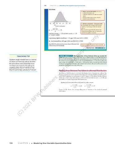
SOLUTION:
1. Draw a normal distribution. Be sure to:
• Scale the horizontal axis.

• Label the horizontal axis with the variable
name.
• Clearly identify the boundary value(s).

• Shade the area of interest.
280 288 296 304 312 320 328 2. Perform calculations—show your work!
290 (i) Standardize the boundary value and use

Distance traveled (yards) Table A or technology to find the desired
area; or
290 −304

z
(i) = =−1.75 ( ii) Use technology to find the desired area
8 without standardizing. Label the inputs you
(C) 2021 BFW Publishers -- for review purposes only.
used for the applet or calculator.

Using Table A : Area for <−z 1.75 is 0.0401. Area for z ≥−1.75

=
is −1 0.0401 0.9599 .
=
−
Using technology: Applet/normalcdf(lower:1.75,upper:1000,mean:0,SD:1)0.9599

=
(ii) Applet/normalcdf(lower:290,upper:1000,mean:304,SD:8) 0.9599

About 96% of Rory McIlroy’s drives travel at least 290 yards. So he Be sure to answer the question that was asked.
is likely to have a clear second shot.
FOR PRACTICE TRY EXERCISE 13.
TEACHING TIP THINK ABOUT IT What proportion of Rory McIlroy’s drives go exactly 290

yards? Because a point on the number line has no width, there is no area directly above
Students might wonder how an interval the point 290.000000000. . . under the normal density curve in the previous example. So,
of values can have any area at all when the answer to our question based on the normal distribution is 0. One more thing: the
290 and x >
areas under the curve with x ≥
290 are the same. According to the normal

the area above every individual value model, the proportion of McIlroy’s drives that travel at least 290 yards is the same as the
is 0. How can a bunch of 0s add up to proportion that travel more than 290 yards.
anything other than 0? Tell them that
they’ll need to take calculus to find out! Finding Areas Between Two Values in a Normal Distribution
How do you find the area in a normal distribution that is between two values? For
instance, suppose we want to estimate the proportion of Gary, Indiana, seventh- graders

with ITBS vocabulary scores between 6 and 9. Figure 2.17(a) shows the desired area

.

under the normal curve with mean µ = 6.84 and standard deviation σ = 1.55 We can

use Table A or technology to find the desired area.
Option (i): If we standardize each boundary value, we get:
66.84 96.84
−
−
z = =− 0.54 z = = 1.39
1.55 1.55

Figure 2.17(b) shows the corresponding area of interest in the standard normal
distribution.
03_StarnesSPA4e_24432_ch02_088_153.indd 134 07/09/20 1:57 PM

134 CHAPTER 2 • Modeling One-Variable Quantitative Data

03_TysonTEspa4e_25177_ch02_088_153_4pp.indd 134 10/11/20 7:47 PM