Page 51 - 2021-bfw-SPA-4e-TE-sample.indd

132 CHAPTER 2 • Modeling One-Variable Quantitative Data

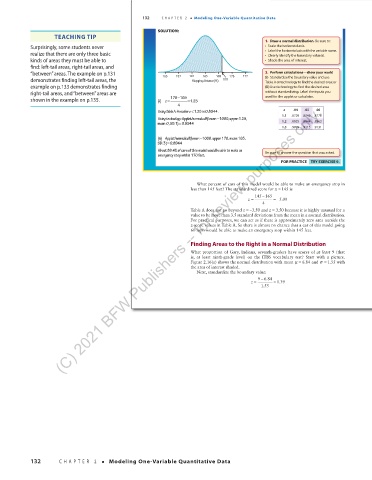
SOLUTION:
TEACHING TIP
1. Draw a normal distribution. Be sure to:
Surprisingly, some students never • Scale the horizontal axis.

realize that there are only three basic • Label the horizontal axis with the variable name.
• Clearly identify the boundary value(s).

kinds of areas they must be able to • Shade the area of interest.
find: left-tail areas, right-tail areas, and
“between” areas. The example on p.131 153 157 161 165 169 173 177 2. Perform calculations—show your work!
demonstrates finding left-tail areas, the Stopping distance (ft) 170 ( i) Standardize the boundary value and use
Table A or technology to find the desired area; or
example on p.133 demonstrates finding (ii) Use technology to find the desired area

right-tail areas, and “between” areas are without standardizing. Label the inputs you
shown in the example on p.135. (i) = 170 −165 =1.25 used for the applet or calculator.
z
(C) 2021 BFW Publishers -- for review purposes only.
4
z

Using Table A : Area for <1.25 is 0.8944. z .04 .05 .06
1.1 .8729 .8749 .8770

Using technology: Applet/normalcdf(lower: −1000,upper:1.25,
mean:0,SD:1)0.8944 1.2 .8925 .8944 .8962
=
1.3 .9099 .9115 .9131
(ii) Applet/normalcdf(lower: −1000,upper:170,mean:165,
SD:3) =0.8944
About 89.4% of cars of this model would be able to make an Be sure to answer the question that was asked.

emergency stop within 170 feet.
FOR PRACTICE TRY EXERCISE 9.
What percent of cars of this model would be able to make an emergency stop in
less than 145 feet? The standardized score for =x 145 is

145 −165
z = =−5.00
4

Table A does not go beyond =−z 3.50 and = 3.50 because it is highly unusual for a

z

value to be more than 3.5 standard deviations from the mean in a normal distribution.
For practical purposes, we can act as if there is approximately zero area outside the
z -score values in Table A So there is almost no chance that a car of this model going
.
60 mph would be able to make an emergency stop within 145 feet.
Finding Areas to the Right in a Normal Distribution

What proportion of Gary, Indiana, seventh-graders have scores of at least 9 (that
is, at least ninth-grade level) on the ITBS vocabulary test? Start with a picture.

Figure 2.16(a) shows the normal distribution with mean µ = 6.84 and σ = 1.55 with
the area of interest shaded.
Next, standardize the boundary value:
−
96.84
= = 1.39
z
1.55
03_StarnesSPA4e_24432_ch02_088_153.indd 132 07/09/20 1:57 PM

132 CHAPTER 2 • Modeling One-Variable Quantitative Data

03_TysonTEspa4e_25177_ch02_088_153_4pp.indd 132 10/11/20 7:46 PM