Page 47 - 2021-bfw-SPA-4e-TE-sample.indd

Lesson 2.5
Normal Distributions:

Finding Areas from Values

LEARNING T AR GET KEY L E AR N I N G TAR G E T S
The problems in the test bank are • Find the proportion of values to the left of a boundary in a normal distribution.

keyed to the learning targets using • Find the proportion of values to the right of a boundary in a normal distribution.

these numbers: • Find the proportion of values between two boundaries in a normal

distribution.
• 2.5.1
(C) 2021 BFW Publishers -- for review purposes only.
• 2.5.2
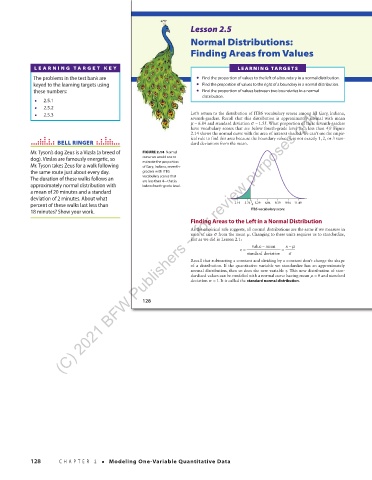
• 2.5.3 Let’s return to the distribution of ITBS vocabulary scores among all Gary, Indiana,
seventh-graders. Recall that this distribution is approximately normal with mean

µ = 6.84 and standard deviation σ = 1.55 What proportion of these seventh-graders
.

have vocabulary scores that are below fourth-grade level (i.e., less than 4)? Figure
2.14 shows the normal curve with the area of interest shaded. We can’t use the empir-

ical rule to find this area because the boundary value, 4, is not exactly 1, 2, or 3 stan-
BELL RINGER dard deviations from the mean.
Mr. Tyson’s dog Zeus is a Vizsla (a breed of FIGURE 2.14 Normal
dog). Vizslas are famously energetic, so curve we would use to
Mr. Tyson takes Zeus for a walk following estimate the proportion
of Gary, Indiana, seventh-
the same route just about every day. graders with ITBS
The duration of these walks follows an vocabulary scores that
are less than 4—that is,
approximately normal distribution with below fourth-grade level.
a mean of 20 minutes and a standard
deviation of 2 minutes. About what
percent of these walks last less than 2.19 3.74 4 5.29 6.84 8.39 9.94 11.49
18 minutes? Show your work. ITBS vocabulary score
Finding Areas to the Left in a Normal Distribution
As the empirical rule suggests, all normal distributions are the same if we measure in

.
units of size σ from the mean µ Changing to these units requires us to standardize,
just as we did in Lesson 2.1 :
−
value mean x − µ
z = =
standard deviation σ
Recall that subtracting a constant and dividing by a constant don’t change the shape
of a distribution. If the quantitative variable we standardize has an approximately
normal distribution, then so does the new variable z This new distribution of stan-
.

dardized values can be modeled with a normal curve having mean µ = 0 and standard

deviation σ = 1 It is called the standard normal distribution

.

.
128
03_StarnesSPA4e_24432_ch02_088_153.indd 128 07/09/20 1:56 PM

128 CHAPTER 2 • Modeling One-Variable Quantitative Data

03_TysonTEspa4e_25177_ch02_088_153_4pp.indd 128 10/11/20 7:46 PM