Page 48 - 2021-bfw-SPA-4e-TE-sample.indd

LESSON 2.5 • Normal Distributions: Finding Areas from Values 129

DEFINITION Standard normal distribution
The standard normal distribution is the normal distribution with mean 0 and standard TEACHING TIP
deviation 1.
Unifying calculations by converting
to z-scores is a powerful tool that is
frequently used in advanced statistics. Lesson 2.5
Repeatedly remind students that the
“standard normal” distribution has mean
–3 –2 –1 0 1 2 3 µ = 0 and standard deviation σ =1.
z-score

Because all normal distributions are the same when we standardize, we can find
areas under any normal curve using the standard normal distribution. Table A in the
(C) 2021 BFW Publishers -- for review purposes only.
back of the book gives areas under the standard normal curve. The table entry for
each z-score is the area under the curve to the left of z.
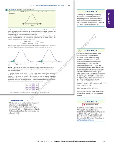
For the ITBS test score data, we want to find the area to the left of 4 under the
normal curve with mean 6.84 and standard deviation 1.55. See Figure 2.15(a). We
start by standardizing the boundary value =x 4:
−
−
value mean 46.84
z = = =− 1.83
standard deviation 1.55
Figure 2.15(b) shows the standard normal distribution with the area to the left of
z =− 1.83 shaded. Notice that the shaded areas in the two graphs are the same.
TEACHING TIP
Looking at Figure 2.15, remind your
students of the transformations
of Lesson 2.2. We are subtracting
=
a constant (themean 6.84) from
every ITBS score and dividing every
2.19 3.74 4 5.29 6.84 8.39 9.94 11.49 –3 –2 –1.83 –1 0 1 2 3 ITBS score by the same constant
(a) ITBS vocabulary score (b) z-score
=
(the standarddeviation1.55). If the
FIGURE 2.15 (a) Normal distribution estimating the proportion of Gary, Indiana, seventh-graders students imagine the thousands of dots
who earn ITBS vocabulary scores less than fourth-grade level. (b) The corresponding area in the stan- that make up the actual ITBS scores piled
dard normal distribution.
up under the normal curve in Figure
z
−
To find the area to the left of =− 1.83, locate 1.8 in the left-hand column of 2.15(a), those dots would be transformed
Table A, then locate the remaining digit 3 as .03 in the top row. The entry to the to look very much like the normal curve
right of 1.8− and under .03 is .0336. This is the area we seek. We estimate that about
3.4% of Gary, Indiana, seventh-graders score below the fourth-grade level on the ITBS in Figure 2.15(b). What can we say about
vocabulary test. Note that we have made a connection between z-scores and percen- the effect of the transformation?
tiles when the shape of a distribution is approximately normal.
Meanof z-scores(ITBS mean–6.84)/1.55 =
=
z .02 .03 .04
−1.9 .0274 .0268 .0262 (6.84– 6.84)/1.55 = 0
=
−1.8 .0344 .0336 .0329 SD of z-scores(ITBS SD)/1.55 =1
−1.7 .0427 .0418 .0409
The shape of z-scores is the same as the
It is also possible to find areas under a normal curve using technology.
shape of the ITBS scores: approximately
normal!
COMMON ERROR
03_StarnesSPA4e_24432_ch02_088_153.indd 129 07/09/20 1:56 PM
Tell students to be careful to find the correct TEACHING TIP
column when reading across Table A. StatsMedic.com
When looking up a left-tail probability that StatsMedic has three blog posts titled
corresponds to z = –1.83, students must go to “Why Do We Standardize Normal
the fourth column from the left, since the first Distributions?,” “Why Bother with z-scores
column is 0.00.
and Table A?,” and “Interpret the z-score
(Like It’s Your Job)” that are relevant to
the content in this lesson. Check it out at
statsmedic.com/blog.

LESSON 2.5 • Normal Distributions: Finding Areas from Values 129

03_TysonTEspa4e_25177_ch02_088_153_4pp.indd 129 10/11/20 7:46 PM